Monday, September 26, 2016

Logging to SysLog

Trace logging of significant events is a fundamental method for debugging and isolating errors encountered. User warnings, pop-up notification boxes, and application-level log files are one way to go. Another; to make use of the standard system log services found on *nix systems. The remainder of this post will some brief information I've recently discovered concerning interfacing with the system log services.

The syslog system import defines the interface:


   extern void syslog (int __pri, __const char *__fmt, ...)


which allows for variable-lengthed argument lists, much like printf. The interface is pretty simple, the first argument specifies a priority or type of log statement; the second, a formatted string in the same form that printf takes.

A simple C

#include <stdio.h>
#include <syslog.h>

int main(int argc, char *argv[]) {
  syslog(LOG_NOTICE,"%s process started", argv[0]);
  sleep(3);
  syslog(LOG_NOTICE,"%s process terminating", argv[0]);
}


Compile and running this example will result in two log entries in the system logs. Determining what log will contain the log statements can be determined by:
1) the log type, and
2) the /etc/syslog.conf file.
Note, that the log type is defined as LOG_NOTICE, and the entry in the syslog.conf file entry;

  *.=info;*.=notice;*.=warn;\
 auth,authpriv.none;\
 cron,daemon.none;\
 mail,news.none          -/var/log/messages

shows that the notice log entries will be evident in /var/log/messages.

Since the files are only accessible to superusers, logging in as root and tailing the log file should show the messages in the same manner as:

# cat /var/log/syslog
.
.
.
Jul  5 20:30:18 riffraff syslogd 1.4.1#18: restart.
Jul  5 20:42:07 riffraff app: ./app process started
Jul  5 20:42:10 riffraff app: ./app process terminating


You can interface with the syslog service using scripts as well.

$ logger -p user.notice "hello again"
# cat /var/log/syslog
.
.
.
Jul  5 20:42:07 riffraff app: ./app process started
Jul  5 20:42:10 riffraff app: ./app process terminating
Jul  5 21:04:06 riffraff lipeltgm: hello again


Pretty slick, huh?
Monday, September 19, 2016

Real-Time Plots with Python -- Bookend

In the past series of posts I focused on using Matlibplot and Python to generate plots.  While the value of plots is not revolutionary, the ease of generating plots with Python and this library makes it worthwhile holstering in 'Ye, Ole Engineering Toolbox'.

I had the sincere opportunity of working with a talented controls engineering department early in my career and acquired a number of life-long experiences.  One of the most significant of which was seeing the significant value in live plotting as an integration and debugging tool.  With dozens of servo controllers, coordinated by multiple sequencers made for a sophisticated system and GDB simply wouldn't cut it for debugging purposes.  Enter 'Simplot', the plotting utility for Matlab, which with relative ease allowed plotting the sequencer state engine as well as the multitude of controller commands and responses.  As the turret moved it wasn't uncommon for the inertia to vibrate or bump a motion controller out of position and stall out the sequencer.  Rendering real-time plots would demonstrate such scenarios with ease and expedite the debugging and iterative development process and made engineering marvels like this a reality:


I took the liberty of simulating the type of plots used, demonstrated in the following video.  


If interested, the Python simulation and plotting is available for your amusement as well.

The plotting however is as easy as the past posts demonstrated.

Cheers.

Sunday, September 11, 2016

Real-Time Plots with Python (Cont)

In the previous posts we've set the stage for some simple Python plotting.  First, we demonstrated the generation of a data set followed by plotting it thereafter.  In the second post, we demonstrated how we could plot 'live' data in real-time.  The astute reader would have observed that over time the 'live' plot will slow down which will result in eventually falling behind plotting the data we're interested in.  This is because an ever-increasing data set will greedily consume the available memory and an ever-increasing data set will eventually grow to an unmanageable size for plotting.
This post will focus on remedying such slow downs by constraining the data set to a manageable size.  We'll also demonstrate some of the multi-plot capabilities of MatlibPlot.

Let's get started;

Reviewing the functionality from the past post, we can plot a 'live', ever-growing data set by something of the following sort:
#!/usr/bin/python
from pylab import *;
import time;
import collections;
import re;

def log(M):
  print "__(log) " + M;

schedEventLoopTime=0.01;
MaxX=50.0;
MaxLen=10;

def test00():
  #--plots a dynamic, continuously growing 2D data set in an autoscaling simple graph
  plt.ion();
  fig=plt.figure(1);
  ax1=fig.add_subplot(111);
  l1,=ax1.plot(100,100,'r-');

  D=[];
  i=0.0;
  while (i < MaxX):
    D.append((i,sin(i)));
    T=[x[0] for x in D];
    L=[x[1] for x in D];
    l1.set_xdata(T);
    l1.set_ydata(L);
    ax1.relim();
    ax1.autoscale_view();
    plt.draw();
    i+=0.10;
    plt.pause(schedEventLoopTime);
  show(block=False);

  plt.close();
#---main---
log("main process initializing");
test00();
log("main process terminating");


A slight modification can increase the plotting performance by constraining the data set to a fixed size; note the use of the collection.
def test02():
  #--plots a dynamic, fixed-length 2D data set in an autoscaling simple graph
  plt.ion();
  fig=plt.figure(1);
  ax1=fig.add_subplot(111);
  l1,=ax1.plot(100,100,'r-');

  D = collections.deque(maxlen=MaxLen);

  i=0.0;
  while (i < MaxX):
    D.append((i,sin(i)));
    T=[x[0] for x in D];
    L=[x[1] for x in D];
    l1.set_xdata(T);
    l1.set_ydata(L);
    plt.ylim([min(L),max(L)]);
    plt.xlim([min(T),max(T)]);
    plt.draw();
    i+=0.10;
    plt.pause(schedEventLoopTime);
  show(block=False);

  plt.close();


The use of the collection allows pre-allocation of a fixed array, appending to a full array will simply push out the oldest value.  The 'live' plot is constrained to a fixed data size, resulting in a plot resembling this;


We'll use the same fixed-sizing concept in a multi-plot example;
def test03():
  #--plots a dynamic, fixed-length 2D data set in an autoscaling multi-plot graph
  plt.ion();
  fig=plt.figure(1);
  ax1=fig.add_subplot(311);
  ax2=fig.add_subplot(312);
  ax3=fig.add_subplot(313);
  l1,=ax1.plot(100,100,'r-');
  l2,=ax2.plot(100,100,'r-');
  l3,=ax3.plot(100,100,'r-');
  time.sleep(3);

  D = collections.deque(maxlen=MaxLen);
  i=0.0;
  while (i < MaxX):
    D.append((i,sin(i),cos(i),cos(i*2)));
    T1=[x[0] for x in D];
    L1=[x[1] for x in D];
    L2=[x[2] for x in D];
    L3=[x[3] for x in D];

    l1.set_xdata(T1);
    l1.set_ydata(L1);

    l2.set_xdata(T1);
    l2.set_ydata(L2);

    l3.set_xdata(T1);
    l3.set_ydata(L3);

    ax1.set_xlim([min(T1),max(T1)]);
    ax1.set_ylim([min(L1),max(L1)]);
    ax2.set_xlim([min(T1),max(T1)]);
    ax2.set_ylim([min(L2),max(L2)]);
    ax3.set_xlim([min(T1),max(T1)]);
    ax3.set_ylim([min(L3),max(L3)]);

    plt.draw();
    i+=0.10;

    plt.pause(schedEventLoopTime);
  show(block=False);
  plt.close();


The result is a 'live' multi-plot that looks like the following;


That's all for now, happy coding.

Monday, September 5, 2016

Real-Time Plots with Python

In my previous post we described plotting data using MatplotLib utilities and Python.  While this may be valuable, it becomes notably more valuable when you can generate 'live' plots during run-time.  In a past employment I worked with a series of controls engineers that utilized real-time data plots to debug and develop a highly complex multi-axis weapons system and it was the first time I understood how a real-time plot of sequence of steps simplified the development effort.

Let's get started.
Unlike the previous post, let's create the data and plot it as it is generated.

$ cat rtPlot 
#!/usr/bin/python
from pylab import *;
import time;

def log(M):
  print "__(log) " + M;

def test01():
  plt.ion();
  fig=plt.figure(1);
  ax1=fig.add_subplot(111);
  l1,=ax1.plot(100,100,'r-');

  time.sleep(2.0);
  D=[];
  i=0.0;
  while (i < 50.0):
    D.append((i,sin(i)));
    T=[x[0] for x in D];
    L=[x[1] for x in D];
    l1.set_xdata(T);
    l1.set_ydata(L);
    ax1.relim();
    ax1.autoscale_view();
    plt.draw();
    i+=0.10;
    plt.pause(1/10.0);
  show(block=True);

#---main---
log("main process initializing");
test01();

log("main process terminating");

The result is a dynamically generated plot that resembles the following:


Tie this plotting routine to a system providing run-time information via a socket, or perhaps monitoring network traffic via pcapture libraries and you've got yourself the foundation of a real-time data monitoring system.

Cheers.

Real-Time Plots with Python

In my previous post we described plotting data using MatplotLib utilities and Python.  While this may be valuable, it becomes notably more valuable when you can generate 'live' plots during run-time.  In a past employment I worked with a series of controls engineers that utilized real-time data plots to debug and develop a highly complex multi-axis weapons system and it was the first time I understood how a real-time plot of sequence of steps simplified the development effort.

Let's get started.
Unlike the previous post, let's create the data and plot it as it is generated.

$ cat rtPlot 
#!/usr/bin/python
from pylab import *;
import time;

def log(M):
  print "__(log) " + M;

def test01():
  plt.ion();
  fig=plt.figure(1);
  ax1=fig.add_subplot(111);
  l1,=ax1.plot(100,100,'r-');

  time.sleep(2.0);
  D=[];
  i=0.0;
  while (i < 50.0):
    D.append((i,sin(i)));
    T=[x[0] for x in D];
    L=[x[1] for x in D];
    l1.set_xdata(T);
    l1.set_ydata(L);
    ax1.relim();
    ax1.autoscale_view();
    plt.draw();
    i+=0.10;
    time.sleep(1/10.0);
  show(block=True);

#---main---
log("main process initializing");
test01();

log("main process terminating");

The result is a dynamically generated plot that resembles the following:


Tie this plotting routine to a system providing run-time information via a socket, or perhaps monitoring network traffic via pcapture libraries and you've got yourself the foundation of a real-time data monitoring system.

Cheers.

Friday, September 2, 2016

Plotting with Python

Scripting languages are incredibly powerful, but more powerful when you can visualize the data you are processing. In this post, we will demonstrate how to quickly plot data sets via Python. Start with installing Python and a plotting utility known as MatplotLib;

$ sudo apt-get install python python-matplotlib

Then, let's start with a classic plot, sin(x);


$ cat pyPlotTest 
#!/usr/bin/python
from pylab import *;
import time;

def log(M):
  print "__(log) " + M;


def test00():
  D=[];
  i=0.0;
  while (i < 50.0):
    D.append((i,sin(i)));
    i+=0.10;

  plt.ion();
  xlabel('radians');
  ylabel('sin(x)');
  grid(True);
  plt.figure(1);
  show();
  T=[x[0] for x in D];
  L=[x[1] for x in D];
  plt.plot(T,L,'b-');
  show(block=True);

#---main---
log("main process initializing");
test00();
log("main process terminating");


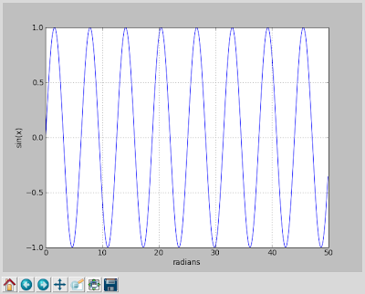
The result is calculating a data set followed by plotting the data and allowing the user to manipulate the plots (e.g. zooming, panning, ...).

Running the script and you'll be presented with the following interactive graph;


The graph is interactive, allowing panning, zooming and such.  It provides similar capabilities as gnuPlot, for those of you familiar with that utility.  This short example demonstrates the simplest of examples.  The library provides a full feature plotting solution for far more advanced plots, such as:


For more detailed features, refer to the MatlabLib site: http://matplotlib.org/contents.html

Cheers.